Kalman filter

The Kalman filter is a recursive method to estimate the state of a linear system with additive process noise. The state variables are observable only by a linear measurement equation with an additive measurement noise. The popularity and flexibility of the Kalman filter are due to the fact that it is the filter with the optimal minimum-mean-squared error (MMSE).

Subsequently, the notation and syntax on kalman-filter.com is presented below. Although the Kalman filter is a discrete filter, the notation for a continuous-time system will be presented first.

Continuous-time state-space

The representation of a linear stochastic system is given by

\[ \dot{\mathbf{x}}(t) = \mathbf{A}(t) \mathbf{x}(t) + \mathbf{B}(t) \mathbf{u}(t) + \mathbf{G}(t) \mathbf{z}(t) \]

where \( t \) represents the time, \( \mathbf{x}(t) \) is the state vector, \( \mathbf{u}(t) \) is the control input, \( \mathbf{z}(t) \) is the input or process noise with known covariance matrix \( \mathbf{Q}(t) \), \( \mathbf{A}(t) \) the system matrix, \( \mathbf{B}(t) \) input matrix and \( \mathbf{G}(t) \) process noise matrix.

The output of such a system, in general, can be written as follows

\[ \mathbf{y}(t) = \mathbf{C}(t) \mathbf{x}(t) + \mathbf{v}(t) \]

where \( \mathbf{C}(t) \) is the measurement matrix that projects the state-space in the measurement-space and \( \mathbf{v}(t) \) adds additive noise with known covariance matrix \( \mathbf{R}(t) \).

Discrete-time state-space

For the use and application of the Kalman filter within a computer, the continous-time system needs to be discretized. For this purpose, this page uses the following notation \[ \mathbf{x}(k) = \mathbf{A}_d(k-1) \mathbf{x}(k-1) + \mathbf{B}_d(k-1) \mathbf{u}(k-1) + \mathbf{G}_d(k-1) \mathbf{z}(k-1) \]

\[ \mathbf{y}(k) = \mathbf{C}(k) \mathbf{x}(k) + \mathbf{v}(k) . \]

With this introduction of the notation, the Kalman filter equations can be hereafter presented.

Kalman filter

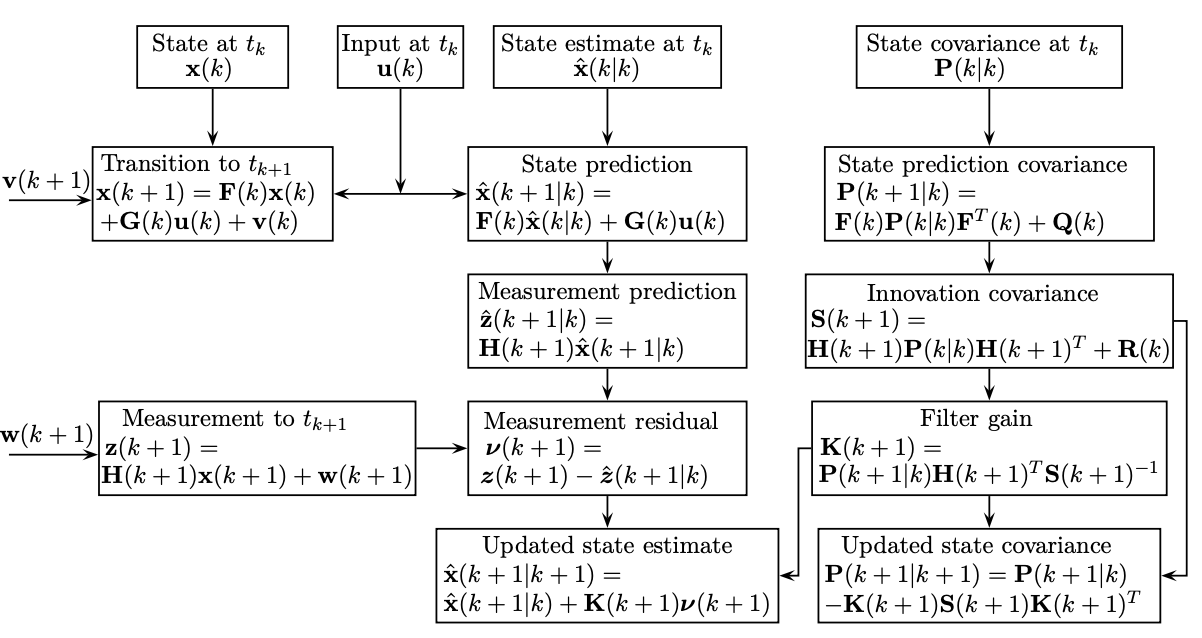
The equations of the Kalman filter consist of five major steps:

State prediction

\[ \mathbf{x}(k|k-1) = \mathbf{A}_d(k-1) \mathbf{x}(k-1) + \mathbf{B}_d(k-1) \mathbf{u}(k-1) \]

State prediction covariance

\[ \mathbf{P}(k|k-1) = \mathbf{A}_d(k-1) \mathbf{P}(k-1) \mathbf{A}_d(k-1)^{T} + \mathbf{Q}_d(k-1) \]

Filter gain

\[ \mathbf{K}(k) = \mathbf{P}(k|k-1) \mathbf{C}(k)^{T} (\mathbf{C}(k) \mathbf{P}(k|k-1) \mathbf{C}(k)^{T} + \mathbf{R})^{-1} \]

Update state estimate

\[ \mathbf{x}(k) = \mathbf{x}(k|k-1) + \mathbf{K}(k) (\mathbf{y}(k) - \mathbf{C}(k) \mathbf{x}(k|k-1) ) \]

Update state covariance

\[ \mathbf{P}(k) = \bigl(\mathbf{I} - \mathbf{K}(k) \mathbf{C}(k) \bigl) \mathbf{P}(k) \bigl(\mathbf{I} - \mathbf{K}(k) \mathbf{C}(k) \bigl)^T + \mathbf{K}(k) \mathbf{R}(k) \mathbf{K}(k)^T \]

Further reading

The Kalman filter is named after the publication of Rudolf Emil Kalman who presented his approach in 1960 in the paper “A New Approach to Linear Filtering and Prediction Problems” [1]. However, the idea was described by other authors several years earlier. Nevertheless, the spread of the concept is attributed to Kalman.

The original derivation of the Kalman filter was via the orthogonality principle. Later, other authors derived the filter in the Bayesian reference frame [2]. The Bayesian derivation is since then the most common because it is more accessible from a didactic perspective.

Unfortunately, the use of the Bayesian derivation leads to the Kalman filter being associated with a Gaussian assumption in both process and measurement noise. However, the Kalman filter is MMSE-optimal without any assumption of Gaussanity [3].

References

[1] Kalman, R. E. (1960). “A New Approach to Linear Filtering and Prediction Problems”. Journal of Basic Engineering. 82: 35–45.

[2] Y. Ho and R. Lee (1964). “A Bayesian approach to problems in stochastic estimation and control”. IEEE Transactions on Automatic Control, vol. 9, no. 4, pp. 333-339.

[3] Uhlmann, Jeffrey & Julier, Simon. (2022). Gaussianity and the Kalman Filter: A Simple Yet Complicated Relationship. Journal de Ciencia e Ingeniería. 14. 21-26. 10.46571/JCI.2022.1.2.