Estimating the state of a dc motor
This example will focus on estimating the angular position \( \theta \), angular velocity \( \dot{\theta} \) and armature current \( i \) of a DC motor with a linear Kalman filter. When modeling DC motors, it is important to mention that certainly nonlinear models are superior to linear ones. For didactic purposes, the following widely used linear model is sufficient for the time being.
Continuous-time system model
The modeling of a DC motor is structured into two parts. The electrical part is modeled with the electrical equivalent circuit and the kinematics with the basic equations of a DC motor.
Electrical system model
The electrical part consists of the armature resistance \( R \) and the inductance of the armature winding \( L \) which are connected in series, and the electromechanical energy converter \( M \) which is the DC motor. The circuit is operated by the voltage source \( V_s \).
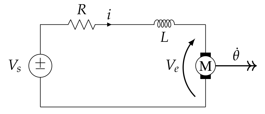
The following equation can be determined using the mesh equation
\[ V_s = L \dot{i} + R i + V_e .\]
The DC motor induces the voltage \( V_e \) that can be regarded linear to the angular velocity \( V_e = K_e \dot{\theta} \) with the motor velocity constant \( K_e \).
Since \( L \dot{i} \) is a differentiating term, we solve for the same and get the following first order differential equation
\[ \dot{i} = \frac{1}{L} V_s - \frac{R}{L} i - \frac{K_e}{L} \dot{\theta} \]
that we will later transfer to the state-space.
Kinematic system model
For the mechanical part, the DC motor is described by the physics of rotations around a fixed axis. It is assumed that the mechanical shaft and the rotated body, i.e. the actuated load, are known and subsumed under the angular mass \(J\).
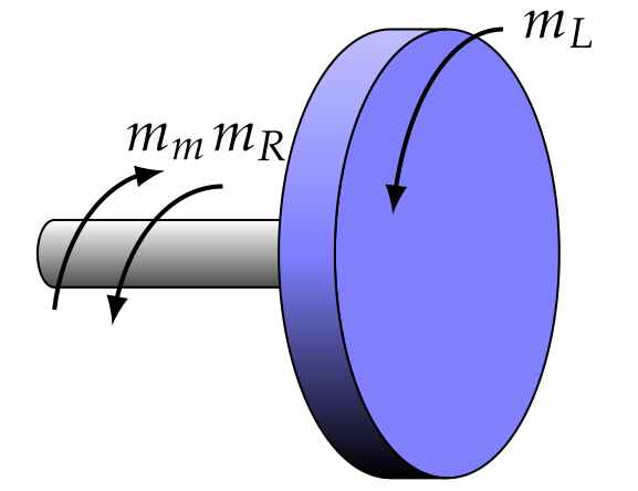
The relationship between the angular acceleration \(\ddot{\theta}\) caused by the net torque is then as follows
\[ J \ddot{\theta} = m_m - m_R - m_L . \]
Where \(m_m\) is the motor torque. The friction torque \( m_R \) and load torque \( m_L \) counteract to the motor torque \(m_m\). For the motor torque \(m_m\) there is a linear relationship to the current \( m_m = K_T i \) that is adjusted by the factor \( K_T\) which is referred to as motor torque constant. The friction torque \( m_R \) is proportional to the angular velocity \( m_R = b \dot{\theta} \) multiplied by the coefficient \( b\). The torque \( m_L \) is the mechanical load torque that is \( m_L = 0 \), if the DC motor is operated without payload, but we will assume later a unknown load torque. Since \( \ddot{\theta} \) is the term with the highest differentiation, we solve for the same and get the following second order differential equation
\[ \ddot{\theta} = \frac{K_T i}{J} - \frac{b}{J} \dot{\theta} - \frac{m_L}{J} . \]
Combined DC motor model
The two upper differential equations can now be transferred into one combined state-space model of the form
\[ \dot{\mathbf{x}}(t) = \mathbf{A} \mathbf{x}(t) + \mathbf{B} \mathbf{u}(t) + \mathbf{G} \mathbf{z}(t) . \]
For this purpose, the kinematic differential equation of second order gets converted into a first-order differential equation by defining \( x_1:=\theta \) as the first state variable and \( x_2:=\dot{\theta} \) as its derivative. Additionally, we model the derivative of the load torque \( m_L \) as an unknown disturbance
\[ \dot{m_L} = z(t), \]
which means we define the load torgue as a third state variable \( x_3:=m_L \). For the first-order electrical differential equation, we can directly define \( x_4:=i \) as the fourth and last state variable. Furthermore, the combined system is only controlled by the voltage supply, i.e.,
\[ \mathbf{u}(t) = V_s. \]
Arranging everything into state-space form, we get
\[ \underbrace{\begin{bmatrix} \dot{\theta} \\ \ddot{\theta} \\ \dot{m_L} \\ \dot{i} \end{bmatrix}}_{= \dot{\mathbf{x}}(t)}= \underbrace{\begin{bmatrix} 0 & 1 & 0 & 0\\ 0 & -\frac{b}{J} & -\frac{1}{J} &\frac{K_T}{J} \\ 0 & 0 & 0 & 0 \\ 0 & -\frac{K_e}{L} & 0 & -\frac{R}{L}\end{bmatrix}}_{=A} \underbrace{\begin{bmatrix} \theta \\ \dot{\theta} \\ m_L \\ i \end{bmatrix}}_{=\mathbf{x}(t)}+\underbrace{\begin{bmatrix} 0 \\ 0 \\ 0 \\ \frac{1}{L}\end{bmatrix}}_{=\mathbf{B}} \mathbf{u}(t) + \underbrace{\begin{bmatrix} 0 \\ 0 \\ 1 \\ 0\end{bmatrix}}_{=\mathbf{G}} \mathbf{z}(t) . \]
For the measurement equation
\[ \mathbf{y}(t) = \mathbf{C} \mathbf{x}(t) + \mathbf{v}(t), \]
we assume we measure the angular position \( \theta = x_1 \) with an absolute encoder, and from this, the measurement matrix follows
\[ \mathbf{C} = \begin{bmatrix} 1 & 0 & 0 & 0\end{bmatrix}. \]
Some notes, the choice of state variables is the part of modeling and it is possible for both another choice and another order. When modeling the load torque \( m_L \), it was assumed that the load torque \( m_L \) is unknown and noisy. Sine the load torque \( m_L \) is not mean-free, it is not possible to set \( \mathbf{z}(t) = m_L\). One practice is therefore to assume the change (i.e. the derivative) to be mean-free and to set the variable as an additional state (here \( x_3 \)).
Discrete-time system model
Discretization of the matrices \(\mathbf{A}_d\) and \(\mathbf{B}_d\) does not yield handy formulations if analytical discretized. Therefore, the discretization is done with the following values \( J=0.0001 \ kg \cdot m^2 \), \(b=0.0001 \ \frac{Nm}{0.5 \cdot rad} \), \(K_T=0.03 \ \frac{Nm}{A} \), \(K_e=0.03 \ V \), \(R=0.5 \ \Omega \), \(L=0.0004 \ H\) and \(T_s=0.1 \ s \) that are later also used for the simulation by using the known equations
\[ \mathbf{A}_d = e^{\mathbf{A} T_s} \]
\[ \mathbf{B}_d = \int^{T_s}_{0} e^{\mathbf{A} \tau} d \tau \mathbf{B} . \]
For the sake of completeness, the discrete system model is \[ \mathbf{x}(k) = \mathbf{A}_d(k-1) \mathbf{x}(k-1) + \mathbf{B}_d(k-1) \mathbf{u}(k-1) + \mathbf{z}(k-1) \]
\[ \mathbf{y}(k) = \mathbf{C}(k) \mathbf{x}(k) + \mathbf{v}(k) . \]
It is worth taking a look at the 3rd state variable \(x_3\) with the load torque \[ m_L(k) = m_L(k-1) + v_{m_L}(k-1) .\] The line is to be understood in such a way that the change of the load torque from time \( k-1 \) to time \( k \) corresponds to gaussian noise, i.e. a random walk. This is the primary modeling choice made here. The rest corresponds to the standard procedure for modeling a DC motor.
Observability
In order to check whether the modeling of the measurement mapping allows to observe all states, one can check the rank of the observability matrix \[ \mathbf{O} = \text{rank} \begin{bmatrix} \mathbf{C} \\ \mathbf{C} \mathbf{A}_d \\ \mathbf{C} (\mathbf{A}_d)^2 \\ \mathbf{C} (\mathbf{A}_d)^3 \end{bmatrix} = 4 . \] In this case, the rank corresponds to the number of degrees of freedom and thus the system is fully observable with the chosen measurement mapping \( \mathbf{C}\).
Determination of the system and measurement noise
There are different ways to determine the process noise. Since here only simulative work is done, all ways would work. In practice, it would be necessary to evalulate more precisely which path and which parameterization should be selected. Here the variance is set to \( \sigma_{m_L}^2 = 2.25 \cdot 10^{-6} \) with \[ \mathbf{Q} = \begin{bmatrix} 0 & 0 & 0 & 0\\ 0 & 0 & 0 & 0 \\ 0 & 0 & \sigma^2_{m_L} & 0 \\ 0 & 0 & 0 & 0 \end{bmatrix} . \] For the calculation of the covariance matrix of the discrete process noise the discretization with zero-order hold is chosen \[ \mathbf{Q}_d = \int^{T_s}_{0} e^{\mathbf{A} \tau} \mathbf{Q} e^{\mathbf{A}^T \tau} d \tau . \] The calculation does not provide a handy result for \( \mathbf{Q}_d \) therefore it is not given here.
The determination of the measurement noise is based on the assumption that the angular position of the dc motor is determined by an absolute encoder with a resolution of 12 bits. This results in 4096 discrete positions, where one position corresponds approximately to an interval length of 0.088 degrees. The variance of the measruement noise need to be set equal to the variance of the continuous uniform distribution \[ \sigma^2_r = \frac{1}{12} ( \frac{2 \pi}{4096} )^2 = 1.96 \cdot 10^{-7} \ \text{rad}^2 . \]
Implementation and results
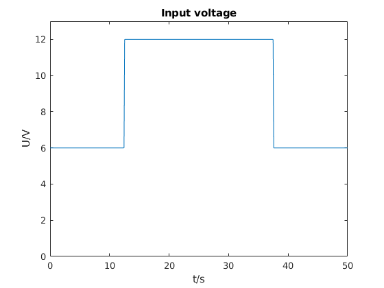
The following results were received by conducting a simulation in MATLAB. To make the simulation more lively and realistic, the input voltage is set to 6 V and in the middle of the simulation to 12 V to mock a controller (see the figure below).
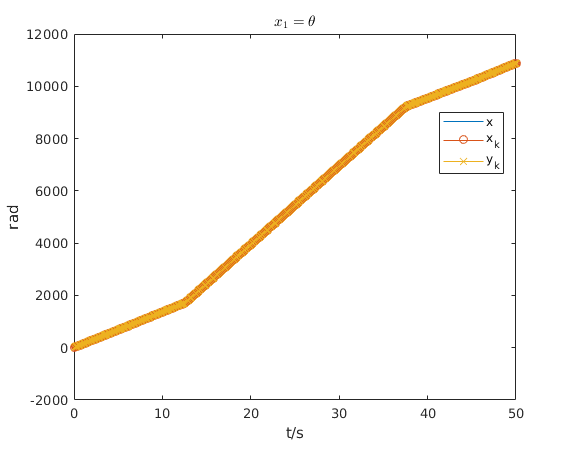
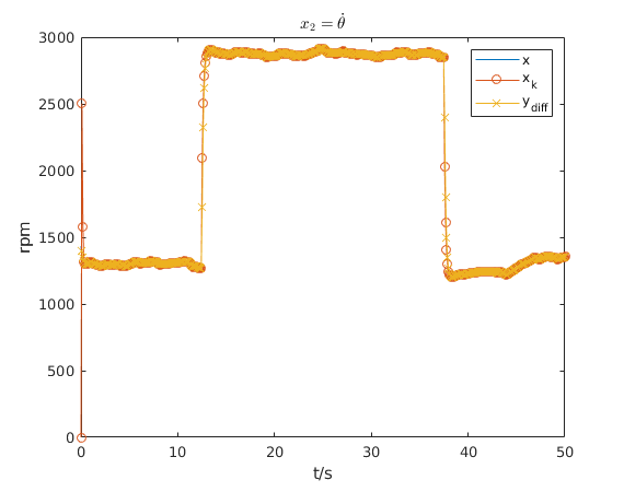
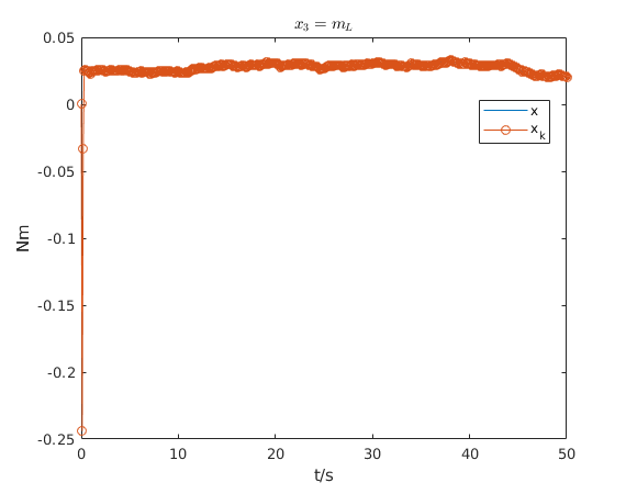
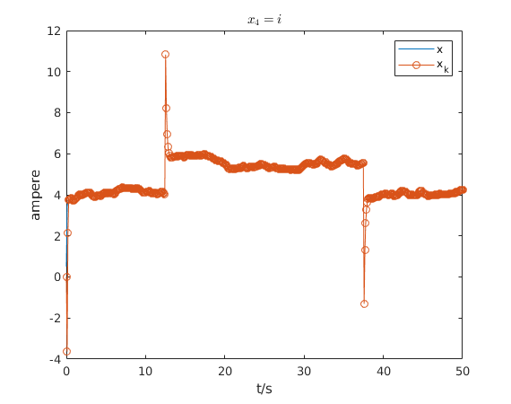
The next four figures shows the course of the estimate of \(\mathbf{x}\) and the ground truth of \(\mathbf{x}\). Additionally, for the first state \(x_1\) the measurements \(y\) are plotted. For the second state \(x_2\), i.e. the angular velocity \( \dot{\theta} \), the approximate derivative \(y_{diff}\) is plotted. Qualitative can be evaluated for all states that the estimate is very close to the true value.
The previous result was mainly qualitative, a widely used quantitative way is to evaluate the estimation error with a metric such as the Root Mean Square Error (RMSE). The next figure shows the RMSE for \( x_1\) and the measurement \(y\). It can be seen that RMSE for \( x_1\) of the Kalman filter matches the RMSE of the measurement \(y\). The main reason is that the measurement noise is very low.
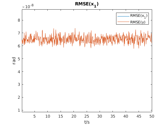
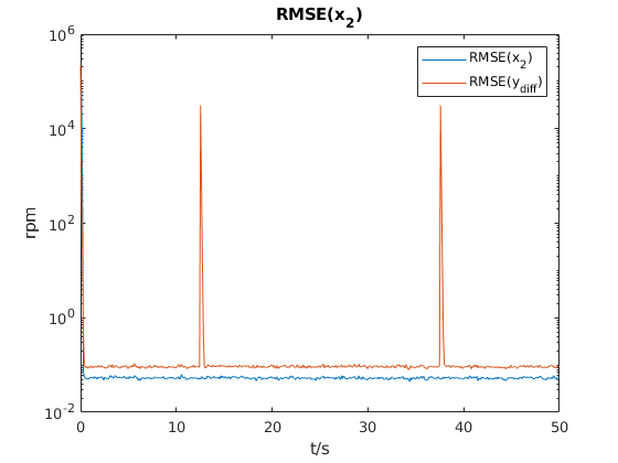
Usually the angular velocity \( \dot{\theta} \) is used to control a DC motor. Without a state estimator, one may be inclined to derive the measured position by approximate derivative and control to this quantity. In the next figure the RMSE for the derived measurement is also shown. It can be clearly seen that the RMSE spikes when the input voltage changes in a jump.
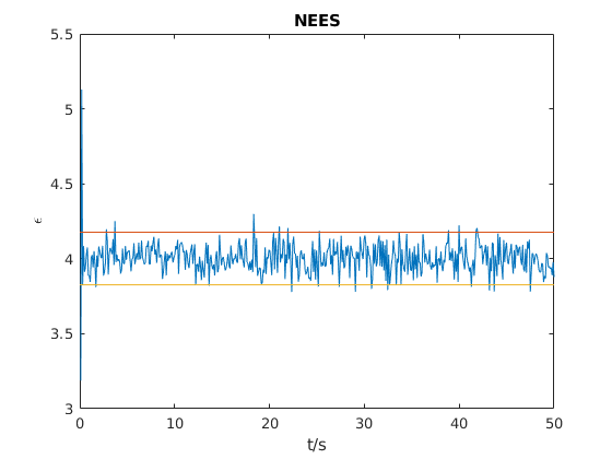
As the last step, the correctness of the simulation can be confirmed by the Normalized Estimation Error Squared (NEES). Since 1000 Monte Carlo runs were performed, a 95% confidence interval \( [3.83;4.18] \) can be determined. The next figure shows the NEES that stays within the confidence interval. Moreover, the mean of the NEES is close to 4 which is the degree of freedom of the used state-space system.
References
The text book from Yaakov Bar-Shalom et al. Estimation with Applications to Tracking and Navigation: Theory, Algorithms and Software is an incredibly useful reference.